Doing Bayesian Data Analysis

Assuming I can keep at it, I’ll be making my way through Kruschke’s Doing Bayesian Data Analysis. Here’s a few concepts he goes through in Chapter 4.

The Bayes factor

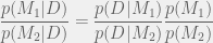
This is a ratio which allows you to compare which out of two models best fits the data. By introducing a binary parameter which determines the choice of model, Bayes’ rule

gives us the Bayes factor

or also

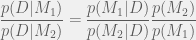
Note that if we have no prior preference between the two models, these ratios are equal.

The Bayes’ factor is useful because on their own scale on the basis of the model – the more complex the model, the lower the absolute value – but this is actually a good thing because by considering the ratio we automatically trade off complexity (when there’s little data) against descriptive value (when the simpler model doesn’t fit the data).

Data order invariance

I don’t get this part – it’s always true that is invariant of the order in which Bayes’ rule is applied, by definition. The factorized rule cited at the end is just the result of applying the definition of data independence given the parameters.

The problem with Bayesian mathematics

Computing the posterior given some new data usually means performing an integral, which, even using approximations, can be computationally intensive (especially since the posterior will be fed into an optimizer). Numerical integration on the other hand would impose a limit on the dimensionality of the model. Thus we winning method is Markov Chain Monte Carlo (MCMC).